Quick Start Guide

This Quick Start Guide gives a fast and simple introduction into PoC. All topics can be found in the Using PoC section with much more details and examples.

Contents of this Page

Requirements and Dependencies
TL;DR
Download
Configuring CaDH on a Local System
Customization
Run a Simulation
Plotting
- Plot ABCI results
- Plot Excel Files

Requirements and Dependencies 

The CaDH is a GUI for coordinating different electromagnetic codes. It also comes with some scripts to ease most of the common tasks. CaDH uses Python 3 as a platform independent scripting environment. All Python scripts are wrapped in Bash or PowerShell scripts, to hide some platform specifics of Darwin, Linux or Windows. See USING:Require for further details.

TL;DR 

git clone https://github.com/Dark-Elektron/CavityDesignHub.git
pip install -r requirements.txt

Navigate to <root>\CavityDesignHub\exe\SLANS_exe\fonts and install all fonts in the folder.
Download ABCI version 12.5 code from here.

cd <root>/CavityDesignHub
unzip ABCI_MP_12_5.zip
robocopy ABCI_MP_12_5 <root>\CavityDesignHub\exe\ABCI_exe /COPYALL /E

CavityDesignHub requires:

The Python 3 programming language and runtime.

CaDH optionally requires:

Git command line tools or
Git User Interface, if you want to check out the latest ‘master’ or ‘release’ branch.

All dependencies are contained in requirements.txt

Download 

The CaDH-Library can be cloned with git clone. GitHub offers HTTPS and SSH as transfer protocols. See the Download page for further details.

Protocol	Git Clone Command
HTTPS	git clone –recursive https://github.com/Dark-Elektron/CavityDesignHub.git
SSH	git clone git@github.com:Dark-Elektron/CavityDesignHub.git

To install the requirements, use

pip install -r requirements.txt

Note

On PyCharm, Right Click on test_plugin and mark directory as Sources Root. A change to this will be considered in later releases.

Configuring CaDH on a Local System 

CaDH currently makes use of other software for analysis. These software are not outrightly open source but could be obtained from the website of the author.

SuperLANS

For eigenmode analysis, SLANS is required. The executable files are included in the cloned repository. There might, however, be a problem with the codes because they use fonts that are not included in the standard Windows OS. To install the fonts, navigate to <root>\CavityDesignHub\exe\SLANS_exe\fonts and install all fonts in the folder.

ABCI

For wakefield analysis, the ABCI code is required.

Download ABCI code from here <https://abci.kek.jp/abci.htm>. ABCI version 12.5 is recommended.
Copy files from the downloaded zip file to <root>\CavityDesignHub\exe\ABCI_exe. This can be done directly on

Windows by copying the files to the specified folder or from the command line using

On Windows

First extract the files from ABCI_MP_12_5.zip

cd <root>/CavityDesignHub
unzip ABCI_MP_12_5.zip

Copy all files in extracted folder to <root>\CavityDesignHub\exe\ABCI_exe

robocopy ABCI_MP_12_5 <root>\CavityDesignHub\exe\ABCI_exe /COPYALL /E

On Linux

cd <folder containing zip file>
unzip ABCI_MP_12_5.zip

Copy all files in extracted folder to <root>\CavityDesignHub\exe\ABCI_exe

Customization 

The GUI theme can be changed by clicking on the drop down menu in the top right corner of the GUI and selecting the desired theme. After this, click on Apply to apply the theme. To save this selection for the next time the software is run, click on Save on the menu bar.

Warning

Several buttons are currently non-functional in this GUI. The software is stillv very much under development but it can do the basic things which, for most design studies, are enough.

Run a Simulation 

To run a simulation, we first need to create a project.

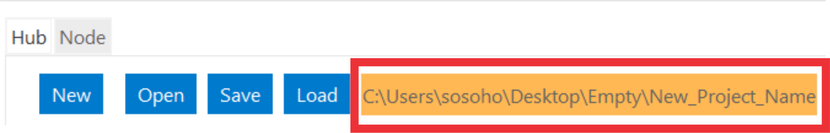
Create New Project 

To create a new project,

Click on New on the menubar.

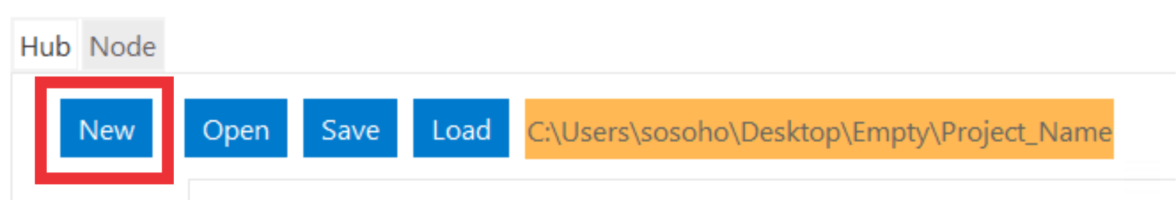
Enter the name of the project and click Enter on your keyboard.

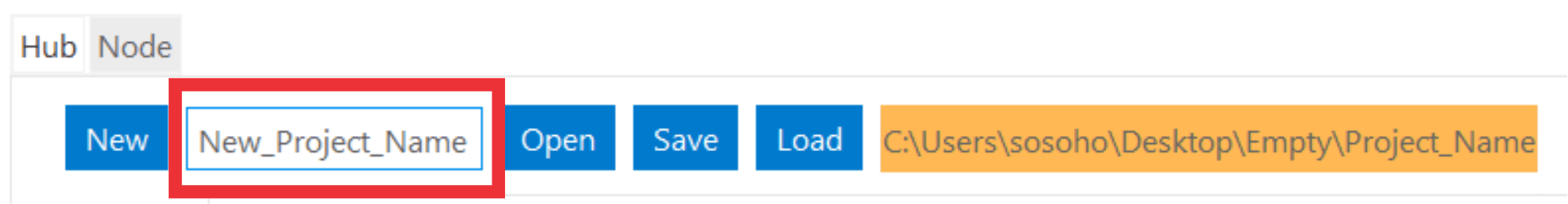
Specify the folder to save the project to.

Now we are ready for our first analysis.

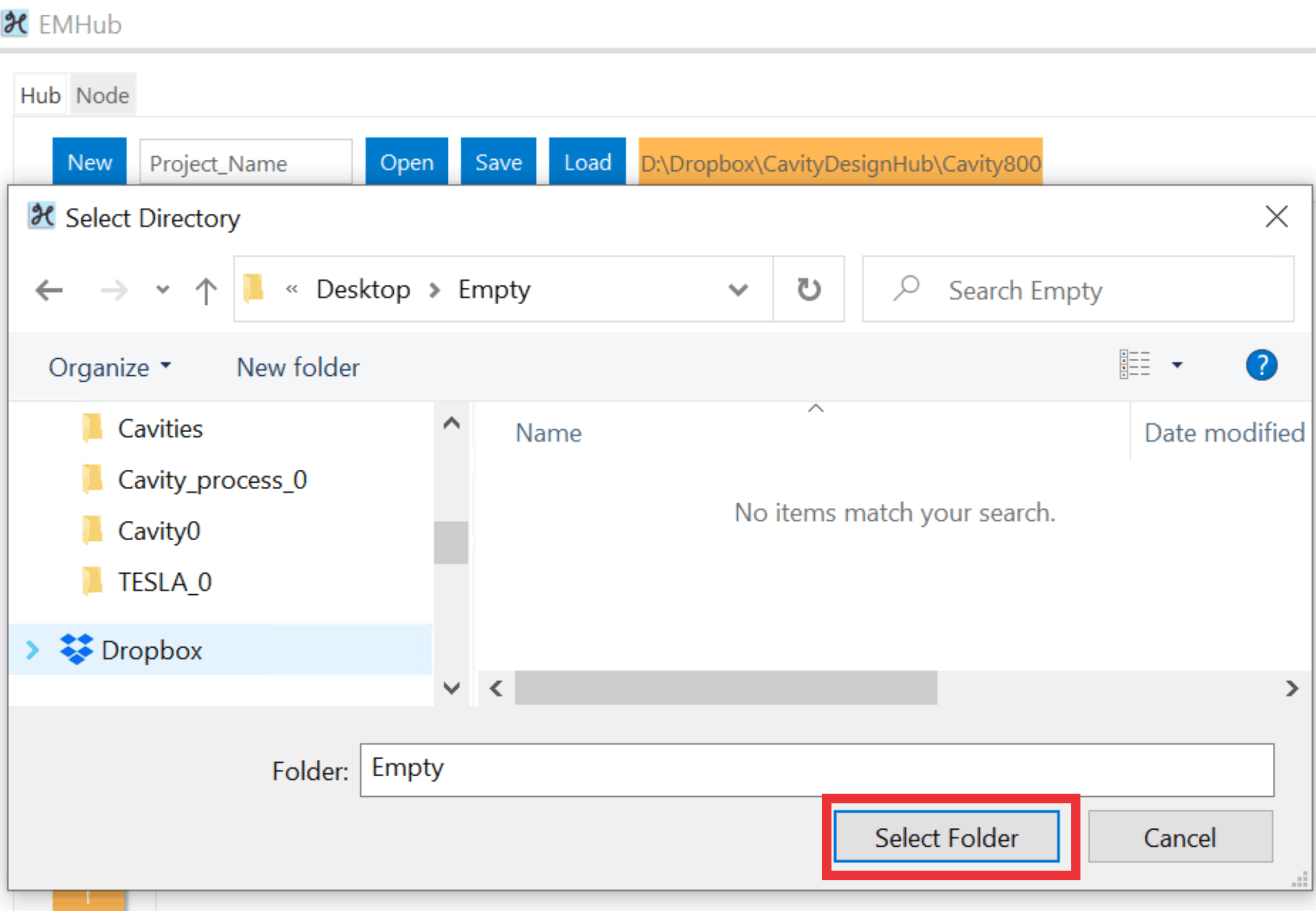
Open Project 

To open a project,

Click on Open on the menubar.
Navigate to the folder containing the project files.
Click on Select Folder.

Once setup is complete, the GUI can be launched by navigating to the folder containing the main.py file. Run the following command from the Windows command line

python3 main.py

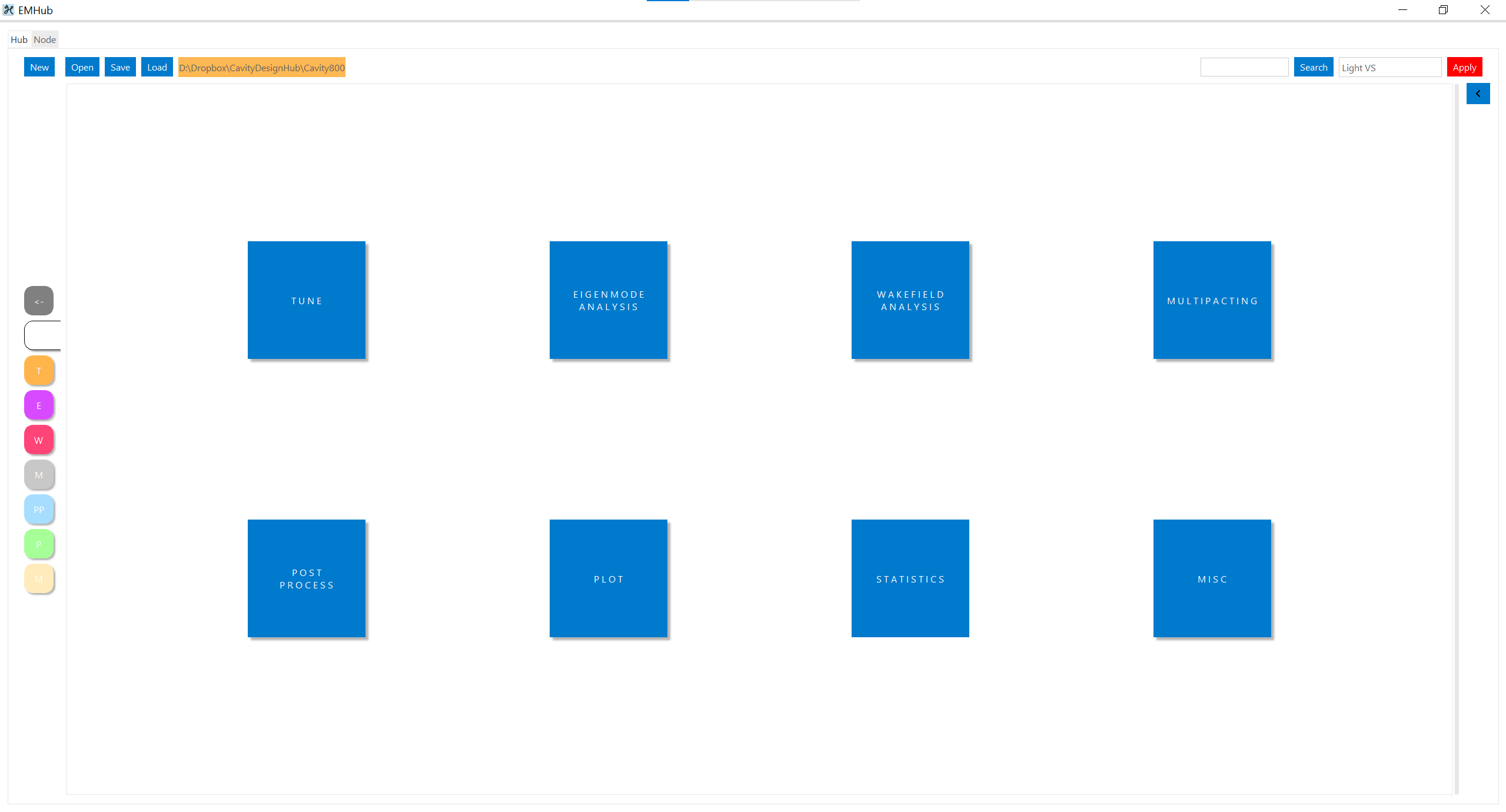
In a Python IDE, open and run main.py directly in the IDE. This opens the GUI as shown in the following figure

Eigenmode Analysis 

First,we are going to run an eigenmode analysis. * | Click on EIGENMODE ANALYSIS. This takes you to another frame which contains different fields and buttons.

There are four major categories on the left pane. These are Cell Geometric Parameters, Cell Parameters, Analysis Settings and Uncertainty Quantification.

Let’s say we wanted to run an eigenmode analysis on the mid cell TESLA cavity ref{} which has geometric dimensions [A, B, a, b, Ri, L, Req] = [] for one eigenmode for single module single mid cell without beam pipes.

For this, we set the boundary conditions of the left and right ends of the cavity to Magnetic Wall En=0 in order to obtain the TM010:math:-pi mode.

Click on Cell Geometric Parameters to expand the input fields

for the geometric parameters if not already expanded.

To enter the geometry for simulation, we create a .json file which contains the dimensions. The structure of the .json file is shown below. The inner cell IC parameters are [A, B, a, b, Ri, L, Req] = [42, 42, 12, 19, 35, 57.7, 103.3, 0]. the left outer cell OC parameters are [A, B, a, b, Ri, L, Req] = [42, 42, 12, 19, 35, 57.7, 103.3, 0], and the right outer cell parameters OC_R are [A, B, a, b, Ri, L, Req, alpha] = [42, 42, 12, 19, 35, 57.7, 103.3, 0]. The outer cell and inner cell dimensions are the same since we are considering just the mid cell of the TESLA cavity. No beam pipes are required so BP is set to none. The frequency FREQ is set to the desired frequency.

{
    "cavity_name":{
        "IC": [
            42,
            42,
            12,
            19,
            35,
            57.7,
            103.3,
            0
        ],
        "OC": [
            42,
            42,
            12,
            19,
            35,
            57.7,
            103.3,
            0
        ],
        "OC_R": [
            42,
            42,
            12,
            19,
            35,
            57.7,
            103.3,
            0
        ],
        "BP": "none",
        "FREQ": 1300
    }
}

Note

Multiple entries are also possible. An example of a .json file that contains two cavities is

{
    "cavity_1":{
        "IC": [...],
        "OC": [...],
        "OC_R": [...],
        "BP": "both",
        "FREQ": 400.79
    },
    "cavity_2":{
        "IC": [...],
        "OC": [...],
        "OC_R": [...],
        "BP": "both",
        "FREQ": 1300
    }
}

Create a file in the project sub directory Cavities and copy the above json formatted text to the file. Change

cavity_name to TESLA. Save the file with a .json extension.
Click on Cell Geometric Parameters to expand the widget if not already expanded.
Click on … and navigate to the file to load the file.
Once loaded, click on Select Shape dropdown. You should see the <cavity_name> in the dropdown.

In our case, <cavity_name> is TESLA. Select it.

Note

If the json file contains more than one cavity’s geometric parameters, they will all be available for selection.

Click on Cell Parameters to expand the widget if not already expanded. Set the fields

No. of Cells and No. of Modules to 1.
Click on Analysis Settings to show the analysis settings widgets.
Leave Freq. Shift as 0, No. of Modes should be left as 1 since

we are only interested in one mode. Leave the polarity as Monopole and if the

Left BC and Right BC should be set to Magnetic Wall En=0. The number

of Processors should be set to 1.
Click on the play button at the bottom right of the panel to run.
Navigate to SimulationData/SLANS/TESLA to see results.

The results are written to SimulationData/SLANS/<cavity_name> If no name was given, the results are saved to SimulationData/SLANS/Cavity0. The quantities that we are interested in could be found in qois.json. This file is writen by Python. The SLANS written files can be viewed using the corresponding executable file in ``<root>/CavityDesignHub/exe/SLANS_exe. The table below shows the files and corresponding executable files to open them.

Executable	File	Remark
genmesh2.exe	`<filename>.geo`	Used to view the geometry and mesh
slansc.exe	`<filename>.geo`
slansd.exe	`<filename>.geo`
slansm.exe	`<filename>.geo`
slanss.exe	`<filename>.geo`
slansre.exe	`<filename>.res`	For most cases, only this executable is used

The geometry could also be entered manually by filling in the values in the field with the corresponding geometric parameter values.

Tune 

In the design of accelerator cavities, we usually want the cavity to operate at a particular frequency. We have six variables to play around with and one variable is reserved for tuning to the desired frequency. In most cases, the equator radius Req is the preferred variable for tuning for mid cell cavities. For the end cells, L is the tune variable. There are several other variations to this. For example, in a single or 2 cell cavity, L or Req could be selected as the tune variable. For cavities with flat-tops, like the Jlab cavities ref{}, l, the length of the flat top section is the tune variable.

In the following example, we will tune Req of the mid cell of a TESLA cavity to operate at a fundamental mode frequency of 1300~MHz. The description of the fields are given in ref{}.

On the homepage of the application, click on TUNE or the side button T. This will navigate

to the Tune frame.
Select Mid Cell as the Cell Type, Variable as Req. Leave Method,

Tuner as PyTune, Left BC and Right BC as Magnetic Wall En=0,

N Cells as 1 and Frequency to 1300.
Enter the geometric parameters to the corresponding fields
Click on the play button to run.

The results are written to SimulationData/ABCI/<filename>. If no name was given, the results are saved to SimulationData/ABCI/Cavity0. The folder contains the geometric properties and quantities of interest on the tuned cavities. They are saved in geometric_parameters.json and qois.json, respectively. This file is writen by Python. They can be viewed with any text editor. The tune results are saved in tune_res.json.

Note

The SLANS software creates a lot of pop ups during the running of any simulation so the system would become unusable for the period of the tuning or eigenmode analysis. It is most noticeable when a large number of cavities are tuned or analysed in one sweep.

Wakefield Analysis 

The process to run wakefield analysis using ABCI is similar to that for eigenmode analysis. The geometry is loaded exactly the same.

Click on … to open the file dialog box and select the .json file

containing the geometric parameters
Click on Cell Parameters to set the number of cells, modules, length of the

left beam pipe, polarity and number of processor. Set Polarity to monopole to

calculate for the longitudinal wakefield analysis, Dipole for transverse wakefield analysis

and Both for both longitudinal and transverse wakefield analysis. Select Both.

The results are written to SimulationData/ABCI/<filename>. If no name was given, the results are saved to SimulationData/ABCI/Cavity0. The quantities of interest are saved to qois.json. This file is writen by Python. The ABCI written files can be viewed using the corresponding executable file in exe/ABCI_exe/TopDrawer for Windows. You can also set the default application for viewing .top files as the ABCI executable file.

Plotting 

The plot module could be used to easily plot the output from the ABCI code. It is also capable of plotting traditional files like Excel files (.xlsx) and text files (.txt). SLANS files output plotting capabilities are not yet available.

Plot ABCI results 

Navigate to the plot frame from the home page by clicking on Plot or P on the side pane.
Change the Code to ABCI if it is not the current text.
Click on … on the column labeled File/Folder. This brings up a folder selection pop-up.

Select the ABCI folder. This should be the default folder when the button is clicked.

If not, navigate to the folder or to any other folder containing ABCI output folder directory.
Click on Select Folder to select folder.
Click on v on the column labeled ID. This lists all the ABCI directories in the selected

directory. Select the results to be plotted. More than one folder can be selected.
Under the Request column, several results could be selected. The selection differs depending on the value of the

selection in the column Polarisation.
A line plot or scatter plot could be made depending on the selection in the column named Axis and

Type. Each plot can also be scaled by changing the values of ScaleX and ScaleY.
Multiple plots could be added by clicking on + at the bottom left of the table or

right-clicking and selecting Add Row.
To change the axes labels and font size, fill out the values in the x-label and y-label

fields. The legend title can also be changed by filling out the values in Legend labels. In case of

multiple plots, the legend labels should be separated by double percentage signs %%.

Plot Excel Files 

Navigate to the plot frame from the home page by clicking on Plot or P on the side pane.
Change the Code to Others if it is not the current text.
Click on … on the column labeled File/Folder. This brings up a file selection pop-up.

Navigate to the Excel file and select it by double clicking or by clicking on Select File.

This loads the Excel file.
Click on ID to select the sheet of interest.
In the column Request, two fields are available. The first is for the variable to plot on the

x-axis and the second for the y-axis. Click on v on either column and select the variables

to be plotted.
Once this is entered, click on Apply to apply changes.

Note

Multiple variables could be selected to be plotted on the y-axis but only one variable can be plotted on the x-axis.

As with the ABCI plots, a line plot or scatter plot could be made depending on the selection in the column

named Axis and Type. Each plot can also be scaled by changing the values of

ScaleX and ScaleY.
Multiple plots could be added by clicking on + at the bottom left of the table or

right-clicking and selecting Add Row.
To change the axes labels and font size, fill out the values in the x-label and y-label

fields. The legend title can also be changed by filling out the values in Legend labels. In case of

multiple plots, the legend labels should be separated by double percentage signs %%.
Once this is entered, click on Apply to apply changes.