Theory

In this section the theory governing the various analysis in this program are introduces. Note that this would not be exhaustive as that would require several semester’s worth of instruction. What is attempted here is to give the fundamental equations, some basic descriptions and method in which the code was written so that one can understand the different line of codes. This is done so that the user can better understand and interpret exactly what results the program outputs and perhaps point out inconsistencies in the theory and code or even ways in which a routine can be optimised for speed and accuracy.

Aceclerator cavity basics

Particle accelerators are devices used for the acceleration of charged particles to high velocities to serve for various purposes. This is achieved using electromagnetic fields. They are specially used for fundamental science research in areas cutting across physics, medicine, material science, and so on. Typical applications today include high energy physics research, biomedical research, radiotherapy, and ion implantation for the manufacturing of semiconductors. Particle accelerators are comprised of several components which include the particle or beam source, a radiofrequency (RF) source, electromagnets, waveguides, resonant cavities, etc.

Resonant cavities are particularly responsible for particle acceleration. Over the last decade, there has been a great deal of advancement in the design and fabrication of resonant cavities. Cavity shapes have evolved from being totally cylindrical in shape, the so-called pillbox cavities, to the widely used (standard) elliptical cavities nowadays. Cavity geometric parameters are selected based on certain desired properties. The so- called cavity figures of merit are used to quantify these desired properties.

Figures of merit in accelerator cavity design

There are several figures of merits that quantify the efficiency and effectiveness of accelerating cavities. These include the quality factor, \(Q\), the shunt impedance, \(R_\mathrm{sh}\), dissipated power, \(P_\mathrm{c}\), stored energy, \(U\), etc.

The quality factor quantifies the ratio of the amount of energy stored in a cavity to the power dissipated at the cavity walls. Mathematically,

\[Q = \omega \frac{U}{P_\mathrm{ds}}.\]

The shunt impedance is another important quantity used to characterise the losses in a cavity. It is given mathematically as:

\[R_\mathrm{sh} = \frac{V_\mathrm{acc}^2}{P_\mathrm{ds}}\]

where \(U\) is the stored energy given as:

\[U = \frac{1}{2} \epsilon_0 \int_V |E|^2 \mathrm{d}V = \frac{1}{2} \mu_0 \int_V |H|^2 \mathrm{d}V.\]

and \(P_\mathrm{c}\) is the power loss given as:

\[P_\mathrm{ds} = \frac{1}{2} R_\mathrm{sh} \int_S |H|^2 \mathrm{d}s.\]

The accelerating voltage is given as

\[V_\mathrm{acc} = \int_0^L E_z (\rho, \phi) e^{j\omega t}\mathrm{d}z.\]

where L is the length of the cavity or beam pipe.

Electromagnetic field theory

Maxwell equations Electromagnetic interactions are represented mathematically with the Maxwell equations.

\[ \begin{align}\begin{aligned}\nabla D = \rho,\\\nabla B = 0,\\\nabla \times H = J + \frac{\partial D}{\partial t},\\\nabla \times E = - \frac{\partial B}{\partial t}.\end{aligned}\end{align} \]

where E is the electric field intensity, and H is the magnetic field intensity, D is the electric flux density, B is the magnetic flux density. They are related by material properties given as follows:

\[ \begin{align}\begin{aligned}D = \epsilon E,\\B = \mu H.\end{aligned}\end{align} \]

Combining the Maxwell equations and using appropriate vector identities result in the wave equations for electric and magnetic fields as follows.

\[\begin{split}\left(\nabla^2 - \frac{1}{c^2}\frac{\partial^2}{\partial t^2}\right)\bigg\{\begin{matrix} E\\H\end{matrix}\bigg\} = 0.\end{split}\]

magnetic permeability and \(\epsilon\) electrical permittivity.

Maxwell eigenvalue problem

The Maxwell Eigenvalue Problem (MEVP) is solved using SLANS cite{SLANS} to evaluate \(e_\mathrm{pk}\), \(b_\mathrm{pk}\), and \(R/Q\). The MEVP is given as

\[ \begin{align}\begin{aligned}\nabla \times \left({\mu}\, \nabla \times E(x)\right) - \lambda(x)\epsilon\, E(x)= 0, & & \lambda = \frac{\omega^2}{c^2},~\mathbf{x} \in \mathbb{R}^7,\\\nabla \cdot E = 0 & & E \in \Omega,\\n \times E = 0 & & E \in \partial \Omega,\end{aligned}\end{align} \]

where:math:mathbf{x} is a vector of the geometric variables describing the domain \(\Omega\) with boundary \(\partial \Omega\), \(\mathbf{E}\) is the electric field, \(\lambda\) a vector of eigenvalues, \(\mu\)

Wakefield analysis

The longitudinal and transverse wake functions \(w_\parallel\) and \(\mathbf{w}_\perp\), respectively, are evaluated using ABCI electromagnetic code cite{ABCI}. They are defined as

\[ \begin{align}\begin{aligned}w_\parallel(\rho, s) &= -\frac{c}{q} \int E_z|_{z=ct-s} \mathrm{d}t,\\\mathbf{w}_\perp(\rho, s) &= \frac{c}{q} \int (\textbf{E}_\perp + c \hat z \times \textbf{B})|_{z=ct-s},\end{aligned}\end{align} \]

where \(s\) is the distance between the leading and a trailing test particle with offset \(\boldsymbol{\rho} = (x, y)\) relative to the \(z\)-axis, and \(z\) is the direction of travel of the particles. The longitudinal (\(Z_\parallel\)) and transverse impedances (\(Z_\perp\)) are evaluated as the Fourier transform of the wake functions thus:

\[ \begin{align}\begin{aligned}Z_\parallel (\omega) &= \frac{1}{c} \int_0^\infty w_\parallel(s) \mathrm{e}^{(i\omega s/c)},\\\textbf{Z}_\perp (\omega) &= \frac{1}{c} \int_0^\infty \mathbf{w}_\perp(s) \mathrm{e}^{(i\omega s/c)}.\end{aligned}\end{align} \]

Theory of multipacting

Multipacting is a phenomenon in resonant frequency structures whereby charged particles are continuously discharged at an exponential rate from the conductor walls of the device. Multipacting occurs only at specific conditions dependent on the alternating field and the wall’s surface properties. More specifically, the emission properties of the wall coupled with the electromagnetic field strength and profile are determinants of multipacting. In accelerating cavities, multipacting occurs mostly at the equator.

For multipacting to occur, two conditions must be satisfied. The first is that the an electron emitted at the cavity wall and driven by the cavity electromagnetic field returns to the same point after an integer number of cycles. Secondly, the impacting electron produces more than one secondary electron cite{Oija}. Different measures could predict Multipacting. The one adopted here is implemented in the 2D code described in cite{Oija, Padamse}. The tools for multipacting analysis are the counter and distance functions. The counter and distance functions are used to predict multipacting.

The counter functions are the electron counter function \(c_N\), enhanced counter function \(e_N\) and total electron counter function \(t_N\). These quantify the number of free electrons remaining after a given number of impacts (20 in this case), the number of secondary electrons and the number of all electrons, respectively, where \(N\) is the maximum number of impacts. The final impact energy \(Ef_N\) of the free electrons is also calculated.

The distance function \(d_N\) defined mathematically as

\[d_N = \sqrt{|x_N-x_0|^2 + \gamma^2|\mathrm{e}^{i\psi_N} - \mathrm{e}^{i\psi_0}|^2}\]

quantifies the distance between the initial point and the last impact point where \((x_0, \psi_0)\), \((x_N, \psi_N)\) are the coordinates of the initial and final position after \(N\) impacts.

Multipacting strongly depends on the surface finish of the cavity wall materials and, therefore, strongly depends on the material’s secondary emission yield curve (SEY). It is quite peculiar because if the energy of the impacting particle is too low or too high, no electron is released. This sets an experimentally determined bound of impact energy for which electrons are released in different materials. Figure ref{fig: sey niobium} shows a typical SEY curve for Niobium.

Sensitivity analysis and uncertainty quantification

Sensitivity analysis is a technique that quantifies the change in a model output induced by an input random variable. It can be considered either on a local or a global scale. For instance, variance-based sensitivity analysis is a form of global sensitivity that uses a ratio of variances to measure the influence of the input parameter on the output. One such method is the Sobol’ decomposition cite{IEEEhowto:Sobol}, and the metric values are the Sobol’ indices. They are calculated using

\[S_j = \frac{\mathbb{V}_j [\mathbb{E}_{\sim j}[Y|\textbf{X}_j]]}{\mathbb{V}[Y]} \in [0, 1]\]

\[ST_{j} = \frac{\mathbb{E}_{\sim j}[\mathbb{V}_{j}[Y|\mathbf{X}_{\sim j}]]}{\mathbb{V}[Y]}\]

where \(S_j, ST_j\) are the main and total Sobol’ indices, respectively, \(\textbf{X}\) is a random vector of independent uniform random variables, and $Y$ is a model output. The first order or main Sobol’ indices \(S_j\) determine the sensitivity of the output due to the variation of only one parameter. On the contrary, the total Sobol’ indices quantify the total effect of an input parameter on the output. They are usually estimated with the (quasi) Monte Carlo (MC) method using~cite{IEEEhowto:Damar Wicaksono}

\[S_j = \frac{\frac{1}{N} \sum_{n=1}^N Y(B)_n \cdot Y(A_B^j)_n - \frac{1}{N} \sum f(A)_n \cdot f(B)_n}{\frac{1}{N} \sum f(A)_n \cdot f(B)_n}\]

\[ST_j = \frac{\frac{1}{N} \sum f^2(A)_n \cdot f(A)_n f(AB^j)_n}{\frac{1}{N} \sum f(A)_n \cdot f(B)_n}\]

where \(A\) and \(B\) are matrices of independent \(N\times D\) samples for \(N\) number of samples and \(D\) number of input parameters, and \(A_B^j\) are matrices built by substituting the \(j^{\mathrm{th}}\) column of \(A\) with that of \(B\). The Latin hypercube sequence (LHS) is used to the build matrices \(A\) and \(B\) here because it is a low-discrepancy sequence. This property of the LHS improves the efficiency of the estimators.

section{Surrogate modelling} MC simulations involve a large number of simulations. Typically, the more simulations, the more accurate the results. To reduce the computational cost required to calculate the Sobol’ indices, surrogate models are used to approximate the model output. A pseudo-spectral approach is taken using polynomial chaos expansion (PCE) given by~cite{IEEEhowto:Xiu07}

\[Y = f(\textbf{X}) = \sum_{\boldsymbol{\alpha} \in \mathbb{N}^M} y_{\boldsymbol{\alpha}} \Psi_{\boldsymbol{\alpha}}(\textbf{X})\]

where \(\Psi_\alpha(\textbf{X})\) represents certain basis functions, \(y_{\boldsymbol{\alpha}}\) are the expansion coefficients to be computed and \(\boldsymbol{\alpha}\) represents multi-indices~cite{IEEEhowto:B. Sudret}. In this work, the geometric parameters are considered to be independent and uniformly distributed. The corresponding orthogonal set of polynomials for this distribution is the Legendre polynomials defined by

\[P_0(x) = 1;~ P_1(x) = x;\]

\[(n+1)P_{n+1}(x) = (2n+1)xP_n(x) - nP_{n-1}(x)\]

for a univariate polynomial. The multivariate polynomial is given as

\[\Psi_{\boldsymbol{\alpha}}(\mathbf{X}) := \prod_{i=1}^N P_{\alpha_i}^{(i)}(X_i)\]

Specifically, according to cite{IEEEhowto:B. Sudret}, to build the PCE, it is sufficient to sample

\[(N-1)\frac{(N+p)!}{N! p!}\]

points, where \(N\) and \(p\) are the dimension and degree of the polynomial, respectively. This implies 1260 simulation samples of the geometric model for \(N=13\) and \(p=2\).

The knowledge of Sobol’s indices significantly speeds up the hook-type coupler’s physically based and mathematically oriented optimization process.

Elliptical Cavity optimization

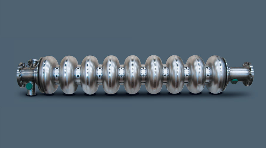
Accelerator cavities consists of cells joined together at either the equator or the iris. Figure {} shows a typical elliptical accelerator cavity. The geometry could be divided into two groups: the mid-cells and the end-cells group. For optimisation purposes, it is computationally cheaper to optimise the groups independently than optimising the entire cavity geometry. Figure {} shows a typical parametrisation of an accelerator cavity. It is important to note that several designers may parametrise the cavity in different ways ref{} and also use different notations.

bibitem{ImageRef} Picture of a nine-cell cavity reprinted from http://www.zanon.com/images/gallery /physics5.jpg, accessed 22/02/2020.